aQRate · Groundwater Monitoring Insights

Educational resource · Environmental monitoring

Groundwater Monitoring: From Well Sampling to Statistical Trend Analysis

Groundwater monitoring turns repeated measurements from a network of wells into evidence of change. Good programs combine well design, consistent sampling, field readings, laboratory analysis and statistical trend tests, because one result rarely shows whether groundwater is changing. This guide walks from the well to the trend, and shows where field data management fits.

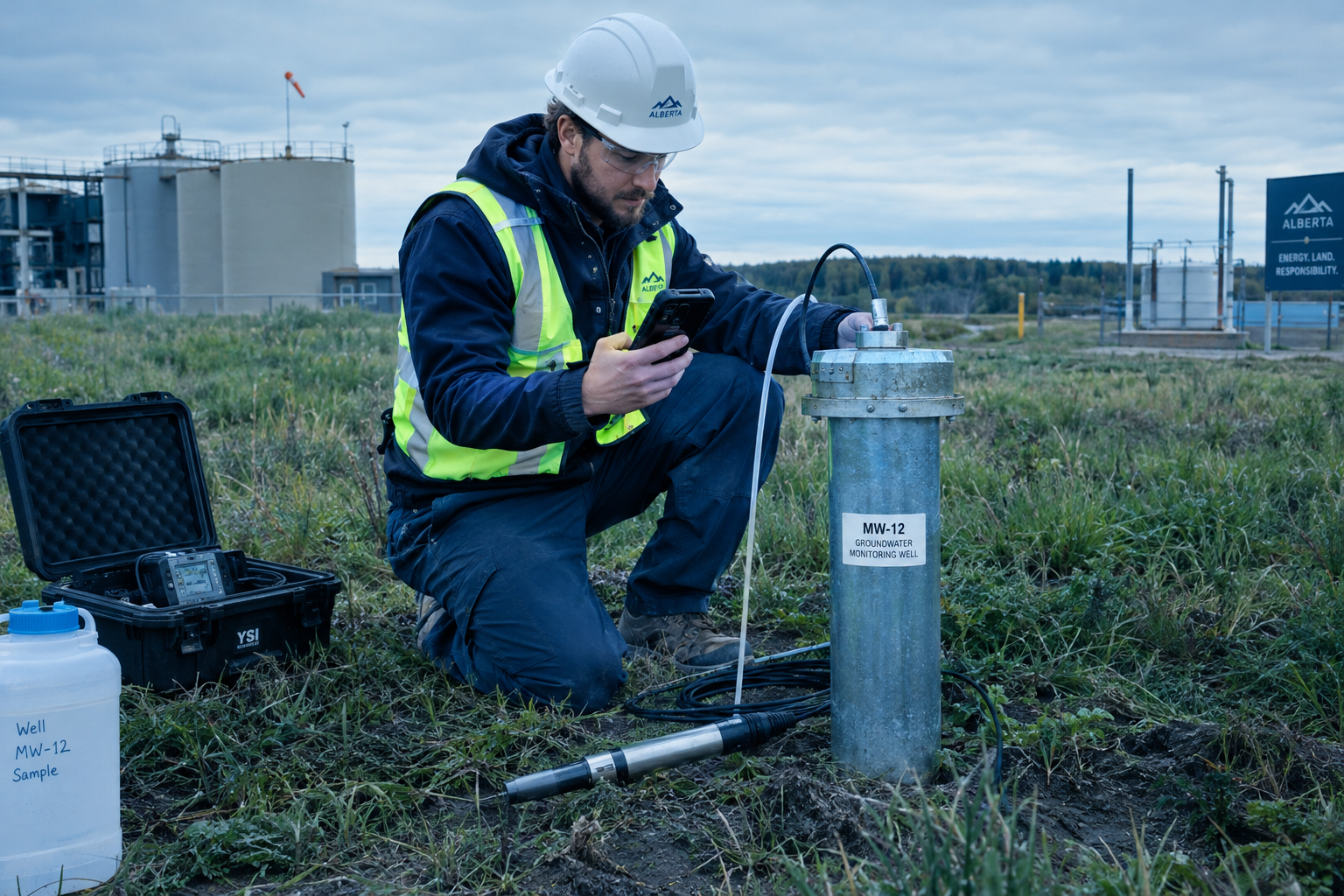
Field technician in a high-visibility vest and hard hat standing beside a groundwater monitoring well, holding a phone and recording readings at the wellhead

A technician records a quarterly field reading at a monitoring well — the first link in the chain this guide follows, from field readings to statistical trend analysis.

Written for
Environmental consultants
Hydrogeologists
Site environmental & compliance managers
Field technicians
Laboratory & data teams
Regulators
Students entering the field

Draws on Government of Alberta, U.S. EPA and USGS publications.

Section 01

What Is Groundwater Monitoring?

Groundwater monitoring is the repeated, comparable measurement of groundwater levels and chemistry from a designed network of wells, over a period long enough to tell real change from natural variability. One sample describes one day; a monitoring program describes a direction.

The purpose is decision support, not data collection for its own sake. Programs are typically run to confirm that conditions remain as expected between events, to detect change from a release or a regional influence early enough to respond, to demonstrate that remediation is performing, and to support reporting to regulators. Alberta frames the assessment and documentation side of this work in its environmental site assessment, Part two: assessment and reporting guidance, while the U.S. EPA’s Statistical Analysis of Groundwater Monitoring Data at RCRA Facilities, Unified Guidance (EPA 530/R-09-007, March 2009) — a technical reference written for RCRA facilities in the United States, not a Canadian requirement — develops the statistical side of exactly this problem: how to turn a sequence of measurements into a defensible statement about change.

01

Set the objectives

Decide what change the program must detect — plume migration, water-level decline, remediation performance — because the objectives set the wells, the frequency and the statistics.

02

Design the network

Place background and downgradient wells, choose screened intervals, and document construction and development so results are comparable over years.

03

Run the sampling events

Measure depth to water and field parameters, purge or low-flow the well, collect samples with QA/QC, and keep custody unbroken.

04

Analyze in the laboratory

Send samples under chain of custody to methods that can report below the decision thresholds, with the lab’s own QA/QC attached.

05

Review the data

Check units, detection limits, non-detects and QC flags before anything is compared, plotted or trended.

06

Test for trends and report

Apply methods suited to noisy, seasonal, censored data, then let a qualified professional read the pattern and decide what it means.

The stages run as a loop, not a line: what the statistics show at the end feeds back into the objectives and the network at the beginning. Synthetic demo dataset. Illustrative only, not customer data. Throughout this guide the running example is a synthetic ten-year quarterly program at three wells — MW-01, MW-02 (the focus well) and MW-03 — with field readings (depth to water, EC, pH, temperature) and a laboratory suite (TDS, major ions, heavy metals).

Section 02

Why Long-Term Records Matter

One result versus a pattern over years: a single quarterly measurement answers “what was the water like on that day”. Whether groundwater is changing is a property of the record, not of a sample.

Individual results move for reasons that have nothing to do with a site: seasonal recharge, a wet or dry year, nearby pumping, purge efficiency, even the calibration of the field probe. When the same well is measured the same way, quarter after quarter, those influences average into a recognizable seasonal texture — and a real change stands out against it. That is why monitoring programs are written for years, not events, and why a record with gaps is weaker than one without, even when the individual numbers look fine.

In the synthetic program, a single depth-to-water reading at MW-02 in one spring quarter tells you where the water table sat that day. Only the full forty-round record shows the slow decline beneath the seasonal rise and fall — the pattern that a trend test can evaluate.

2.9 m3.6 m4.2 m4.9 m5.6 mYr 1Yr 3Yr 5Yr 7Yr 9one quarterly result

Depth to water at MW-02 across forty quarterly rounds: the seasonal saw-tooth repeats, and the slow year-over-year rise is visible only against it.

Conceptual illustration. Synthetic demo dataset. Illustrative only, not customer data. The highlighted point marks how little one quarterly result can say on its own.

Reading the figure: each dot is one quarterly depth-to-water measurement at the focus well, in metres below the measuring point. The dashed line is the Theil-Sen slope of the synthetic series. The same logic applies to chemistry: EC, TDS and metals are judged against their own history, not against one afternoon.

Section 03

A Monitoring Program, End to End

A monitoring program is a cycle of connected activities: objectives, network design, the sampling event, the laboratory, data review, statistics, and the report — with every stage feeding the next.

the report feeds back into the next round’s objectives1Objectives2Networkdesign3Samplingevent4Laboratory5Datareview6Statistics7Report
1Objectivesstage 1 of 72Network designstage 2 of 73Sampling eventstage 3 of 74Laboratorystage 4 of 75Data reviewstage 5 of 76Statisticsstage 6 of 77Report

The end-to-end program cycle: objectives, network design, sampling event, laboratory, data review, statistics and report, looping back to refine the objectives.

Conceptual illustration. Each stage is covered in its own section of this guide — wells (04), sampling (05), data review (06), trend tests (08) and workflow (12).

Weakness at one stage weakens all the others. A well-placed network with a sloppy sampling event produces results that cannot be compared between rounds; a flawless dataset that never reaches a proper trend test never becomes evidence of change; and a strong statistical result in a report that omits units, detection limits or QA/QC context cannot be checked by a reviewer. Alberta’s assessment and reporting guidance and the EPA Unified Guidance (a U.S. technical reference, not a Canadian requirement) both organize monitoring around this loop, each from its own jurisdiction’s side of it.

Section 04

Wells and Network Design

A monitoring network answers questions only if its wells are placed and built with those questions in mind: background wells to define the reference, downgradient wells to catch change, and screened intervals that sample the water you mean to test.

Background and downgradient wells

Background wells sit upgradient or outside the influence being monitored, and they define what “normal” looks like at the site — naturally occurring metals, regional salinity, seasonal water levels. Downgradient wells sit along the expected flow path , where a release would travel. A result at a downgradient well is read against the background wells: a difference is only meaningful when the reference is defined.

Screened interval

The screened interval is the open section of the well through which water enters. A shallow screen and a deep screen in the same location sample different water, so results from different intervals are not comparable. The interval is chosen against the aquifer unit of interest and the depth of the potential impact, and it is recorded with every result — a concentration without its interval is a number without a location.

Construction and development

Casing, screen, sand pack and annular seal keep the well from connecting water zones that should stay apart; a secure, marked surface completion protects the measuring point. Development — surging and bailing or pumping until the water runs clear — removes drilling fluids and fine sediment so the first samples represent the aquifer rather than the borehole. For well construction practice in Alberta, see Alberta Agriculture and Irrigation’s Monitoring well construction, installation and development (AGDEX 096-51, updated June 2024) — note its scope is monitoring wells at confined feeding operations, so it is a practical reference, not a universal standard.

Ground surfaceWater table (illustrative)Groundwater flowMW-01background, upgradientMW-02downgradient, focus wellMW-03downgradient, farthersource area (monitored)screenscreenscreen

Cross-section of a small monitoring network: an upgradient background well, a source area, and two downgradient wells, with the water table and screened intervals shown.

Conceptual illustration, not a real site. Flow direction and well placement follow the conceptual site model, which is revised as results come in.

Section 05

Field Measurements and Sampling

Four field readings travel with every sample: depth to water, EC, pH and temperature. They are cheap, immediate and repeatable — and each of them tells you one thing well and something else poorly.

Field readingWhat it can tell youWhat it cannot tell you
Depth to waterThe position of the water table and how it moves between events; the reference for every other reading and for contouring flow direction.Water quality. Affected by barometric pressure, nearby pumping, the tide of the season, and the exact measuring point used.
Electrical conductivity (EC)A quick field proxy for total dissolved solids; a stable-reading check that purging has finished; a sensitive trend indicator.Which ions are present. Temperature-dependent unless compensated, and diluted or concentrated by sampling itself.
pHWhether the water is acidic or alkaline; context for metal solubility and whether samples were preserved correctly.A precise regulatory comparison on its own — field probes drift with calibration and temperature, and the laboratory value governs.
TemperatureEC compensation, recharge indications, and a purge-stabilization check alongside EC and pH.Much alone. It swings with season, depth and the sun on the flow cell, and it is never a compliance number.

Purging and low-flow sampling

Water standing in a casing is not the water in the aquifer, so a sample is taken after purging the well — traditionally by removing casing volumes, more recently by pumping at a low rate with minimal drawdown. In Low-Flow (Minimal Drawdown) Ground-Water Sampling Procedures (EPA/540/S-95/504, 1996 — a U.S. technical reference), low-flow sampling means a low pumping rate, water-level drawdown kept small, and samples collected only once field readings stabilize. The readings in the table above are the stabilization criteria, not decoration.

QA/QC samples and chain of custody

A monitoring round carries its own quality controls: field duplicates to check sampling precision, equipment or trip blanks where blank contamination is a concern, and calibration checks before the day starts. Chain of custody — who held each sample, when, and under what condition — is what makes a laboratory result traceable to a place and a time. The USGS National Field Manual, Chapter A4: Collection of Water Samples (version 2.0, 2006 — a technical reference) covers the field procedures in detail.

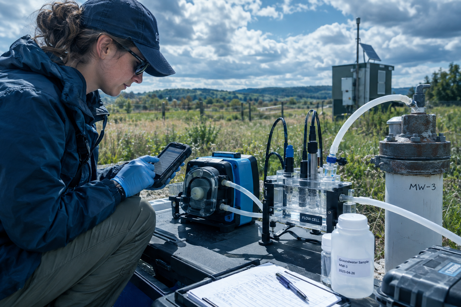
Illustration of low-flow groundwater sampling at a monitoring well: a small pump tubing running to a flow cell measuring EC, pH and temperature, with a sampler recording stable readings in a notebook

Conceptual illustration of a low-flow setup: depth to water is held near static, the pump discharges gently through a flow cell, and the sample is collected only once EC, pH and temperature have stabilized. Illustrative, not a real sampling event.

Section 06

A Concentration Is Not a Conclusion on Its Own

A laboratory number becomes evidence only after its units, its detection limit, its quality context, the site background and the applicable guideline comparison have all been checked — in that order.

Units

A result in mg/L is a thousand times a result in µg/L of the same substance. Results in mixed units, or from different analytical methods, are never directly comparable — a spreadsheet will happily average them anyway.

Detection limits and non-detects

A result reported below the method detection or reporting limit is a censored value, not a zero. How non-detects are treated — substituted, flagged, or handled with methods built for censored data — changes what a trend test sees. A reporting limit that sits above the decision threshold can hide the question entirely.

Background

Naturally occurring substances such as metals can be present without any release. Background wells (Section 04) are how a program tells natural presence from site influence.

Comparison with guidelines

Whether a concentration merits action depends on jurisdiction, land use, exposure pathways, aquifer use and the current edition of the applicable guidelines. In Alberta, the Alberta Tier 1 Soil and Groundwater Remediation Guidelines (June 2024) are part of that framework; which values apply, and whether they are exceeded, is a professional and regulatory judgment — not a lookup on this page.

Hypothetical example — invented values, not real site data

Suppose a laboratory reports arsenic at 12 µg/L in a quarterly sample from MW-02. Before that number means anything:

12 µg/L
arsenic, one quarterly sample, MW-02 — of … what, where, when, how measured?
Unitsµg/L, not mg/L — mixed units are never directly comparable.
Sample ID & datematch the field record before anything else.
Reporting limitwell below 12 µg/L, so the result is a real detection, not an estimate.
QA/QC flagscheck the batch the sample travelled with.
Background & historysame quarter’s background wells, and the same well’s own record.
Guideline comparisonjurisdiction, land use and aquifer use — a professional judgment.

No single step is hard. Skipping any of them is how a number becomes a headline.

Section 07

Why Groundwater Data Breaks Simple Trendlines

A spreadsheet’s default least-squares trendline assumes data that is independent, roughly normal, and untroubled by seasons. Groundwater data is none of those things — it is noisy, seasonal, outlier-prone and frequently censored.

Seasonal recharge moves water levels and chemistry on a fixed annual rhythm. Sampling adds noise: purge behaviour, probe calibration, turbidity. Outliers appear for real physical reasons — a high-turbidity event can mobilize metals for one quarter. And non-detects are censored values, not zeros, so the residuals are not normal either. A least-squares line drawn through that mixture answers a question the data never asked. The EPA Unified Guidance (EPA 530/R-09-007, March 2009) — written for RCRA facilities in the United States, not legally enforceable, and included here as a technical reference only — devotes most of its length to exactly these failure modes.

5736807878941001Yr 1Yr 3Yr 5Yr 7Yr 9seasonal outlier quarter

EC at MW-02 across forty quarterly rounds: the seasonal saw-tooth dominates, one high quarter stands out, and the least-squares line bends toward the outlier instead of describing the record.

Conceptual illustration. Synthetic demo dataset. Illustrative only, not customer data. A robust fit to this series is shown in Section 08.

Section 08

Mann-Kendall and Theil-Sen in Plain Words

Two non-parametric methods carry most of the load in groundwater trend work: one asks whether there is a direction at all, the other estimates how steep it is.

The Mann-Kendall test answers

“Have these ordered measurements been going up or down, more than chance alone would produce?”

It works on ranks, not raw values, so it does not care that the data is skewed or censored, and it can handle non-detects as censored observations rather than forcing them into fake zeros. Its output is a direction and a confidence statement — a detected increasing trend at a stated significance level — not a magnitude, and not a cause.

The Theil-Sen slope answers

“If there is a trend, how fast is it moving — in real units, per quarter or per year?”

It is the median of the slopes between every pair of points, so a single wild quarter cannot drag it. Because the estimate is a median of pairwise slopes, it stays in the units of the measurement — for example, µS/cm of EC per quarter — which is what a report needs in order to say something physical.

-50194439683927Yr 1Yr 3Yr 5Yr 7Yr 9extreme quarter

Solid cyan: Theil–Sen robust slope · dashed red: least-squares line pulled by the outlier · dots: quarterly iron results (µg/L)

Iron at MW-02 with one extreme quarter: the least-squares line (dashed) tilts up toward the outlier, while the Theil-Sen line (solid) holds flat across the record.

Conceptual illustration. Synthetic demo dataset. Illustrative only, not customer data. Both lines are computed from the plotted points; the robust slope is the one that survives the outlier.

Assumptions and cautions

  • Independence: consecutive quarters at the same well are often correlated (serial correlation), and the EPA Unified Guidance warns that autocorrelation inflates the apparent significance of a trend. Test for it, space out events, or account for it.

  • Seasonality: a strong seasonal cycle can masquerade as trend. Seasonal forms of the test, or season-blocked analysis, handle it — the Unified Guidance covers seasonal Mann-Kendall directly.

  • Rounds needed: direction cannot be established from a handful of results. A few years of consistent quarterly rounds is the realistic minimum for a defensible statement.

  • Adequacy of the record: a trend test describes the record it was given — gaps, changed laboratories or changed methods weaken every conclusion drawn from it.

What they do not tell you

Neither test assigns a cause. A detected trend does not say where a change came from — a regional decline, a new upgradient activity, sampling artifact or a real release — and it does not decide whether a regulatory limit is breached. That interpretation belongs to a qualified professional reading the full record: hydrogeology, background wells, QA/QC context and the applicable regulatory framework. For trend methodology in environmental data generally, see Helsel, Hirsch, Ryberg, Archfield and Gilroy, Statistical Methods in Water Resources (USGS Techniques and Methods 4-A3, 2020 — a technical reference).

Section 09

Three Patterns to Read in a Monitoring Record

Most of what a monitoring record shows falls into three shapes: a steady regional movement, a sudden step at one well, and noise with no trend at all. Each is read differently — and none is a conclusion by itself.

Pattern 1 — A steady regional trend, moving together

Depth to water at MW-02 rises slowly across the ten-year record while the seasonal saw-tooth repeats. When EC and TDS rise in step with the water-table decline, the three series corroborate each other: the fields move as one, which is the signature of a regional influence rather than a local event.

2.9 m3.6 m4.2 m4.9 m5.6 mYr 1Yr 3Yr 5Yr 7Yr 9

Depth to water (m) at MW-02 rises across the forty-round record, with a visible seasonal cycle on top.

Conceptual illustration. Synthetic demo dataset.

5736807878941001Yr 1Yr 3Yr 5Yr 7Yr 9

EC (µS/cm) at MW-02 rises across the forty-round record, with a visible seasonal cycle on top.

Conceptual illustration. Synthetic demo dataset.

398471544616689Yr 1Yr 3Yr 5Yr 7Yr 9

TDS (mg/L) at MW-02 rises across the forty-round record, with a visible seasonal cycle on top.

Conceptual illustration. Synthetic demo dataset.

Pattern 2 — A step change at one well

Arsenic at MW-02 sits on a stable baseline for the first five years, then steps sharply upward in Year 6 and stays elevated. A step is a different shape from a slope: it is read as a change in regime at that well, and it is what a quarter-over-quarter review of plotted data is meant to catch.

-37172636Yr 1Yr 3Yr 5Yr 7Yr 9step in Year 6

Arsenic at MW-02 holds a stable baseline for Years 1–5, then steps to a higher, noisier level from Year 6 onward.

Conceptual illustration. Synthetic demo dataset. Illustrative only, not customer data. No cause is stated — source, sampling artifact and regional change are all possibilities a professional reviews.

Pattern 3 — A noisy analyte with no real trend

Iron at MW-02 swings widely quarter to quarter — but a Mann-Kendall test on the full record finds no statistically significant direction. This is the pattern that punishes eyeballing: plotted raw, it looks like it is climbing somewhere; tested properly, it is flat.

23101178256334Yr 1Yr 3Yr 5Yr 7Yr 9

Iron at MW-02 swings across a wide band for ten years, and the robust trend test finds no significant direction — noise, not trend.

Conceptual illustration. Synthetic demo dataset. Illustrative only, not customer data. Chasing the peaks of a series like this is how false alarms start.

The charts above come from the synthetic ten-year quarterly program (three wells, MW-02 as the focus well). They are conceptual illustrations: no cause is stated, and deciding what any pattern means for a site belongs to a qualified professional reviewing the full record and the applicable regulatory framework. Synthetic demo dataset. Illustrative only, not customer data.

Section 10

What a Monitoring Result Must Carry

A single laboratory value is useless to the next reviewer unless it arrives welded to the context that produced it. Traceability is a property of the record, and it is what lets this year’s data be compared with last year’s.

Well IDDate & timeDepth to waterLaboratory & methodSample IDField readings (EC, pH, temp)UnitsDetection limitQA/QC flagsOne reviewable, comparable resultreport readyevery link travels with the value — one missing link weakens the chain
Well IDDate & timeDepth to waterField readings (EC, pH, temp)Sample IDLaboratory & methodUnitsDetection limitQA/QC flagsOne reviewable, comparable resultreport readyevery link travels with the value

Every monitoring result must travel with its well ID, date and time, depth to water, field readings, sample ID, laboratory and method, units, detection limit and QA/QC flags — a chain from the well to a reviewable number.

Conceptual illustration of the traceability chain. A result missing any link — a sample ID without a date, a concentration without units — weakens every comparison and trend built on it.

The U.S. EPA’s field sampling quality-control practice treats this documentation as a quality measure in its own right, and the EPA Unified Guidance builds its statistical methods on the assumption that the record behind each point is intact. In practice, the chain above is also the checklist for the data-review stage of Section 12: anything missing becomes a flag before a number reaches a chart.

Section 11

The Hard Part Is Connecting the Data

A decade-long program does not generate one dataset. It generates thousands of them: field notes, laboratory reports, spreadsheets, emails — created by different people, in different formats, across different years. The information-management problem, not the statistics, is where records get lost.

In practice the failure modes are ordinary. A depth-to-water reading stays in a waterproof notebook and never reaches the spreadsheet. A laboratory PDF is attached to an email thread rather than to the well it came from. Two versions of the same project file differ by one column. Each is a small thing; each breaks a link in the chain from Section 10. And one distinction gets quietly lost along the way: a missing data point and a result that was measured but failed a quality-control check are different data-quality conditions — one is a gap, the other is a measurement whose reliability is in question — and they must not be treated as equivalent, because a blank and a flag tell a reviewer opposite stories.

Section 12

Design the Data Workflow Around the Sampling Event

The sampling event — one crew, one well, one afternoon — is the atom of a monitoring program. A workflow designed around it keeps the record connected from the plan to the report.

01PlanBefore anyone goes to the well.steps below02CollectAt the wellhead, on the day.steps below03ValidateWhen the laboratory data lands.steps below04ReportWhen the record becomes evidence.the report a reviewer can followreview loops: validation sends questions back to planning
01PlanBefore anyone goes to the well.steps listed below02CollectAt the wellhead, on the day.steps listed below03ValidateWhen the laboratory data lands.steps listed below04ReportWhen the record becomes evidence.the report a reviewer can followreview loops between phases

The four-phase workflow — plan, collect, validate, report — with review loops that send validation questions back into planning before the next round.

Conceptual illustration. The phases are not strictly sequential in practice; the loop is where a monitoring program learns from its own record.

Phase 01

Plan

Before anyone goes to the well.
  • Write the objectives and the wells that answer them

  • Set frequency, analytes and field readings

  • Define QA/QC samples and the review rules

Phase 02

Collect

At the wellhead, on the day.
  • Measure depth to water first, every event

  • Purge or low-flow to stable readings

  • Record sample IDs, times and custody as you go

Phase 03

Validate

When the laboratory data lands.
  • Match each result to its well, date and sample ID

  • Check units, detection limits and QC flags

  • Keep missing and QC-failed results distinct

Phase 04

Report

When the record becomes evidence.
  • Run trend tests suited to noisy, censored data

  • Read patterns against background wells

  • Produce the report a reviewer can follow

The phases are not sequential in practice — validation raises questions that send the next planning round back to the well, and a report is only the last of many review loops. What the phases protect is the connection: the reading taken at the wellhead stays attached to the sample that became it.

Section 13

Where Digital Field Data Management Fits

Everything before this section — the wells, the sampling, the statistics, the qualified professional’s judgment — stays exactly as it is. Digital field data management’s role is narrower: keeping the record connected, and doing the arithmetic on it.

What aQRate provides

aQRate is a field data collection and management platform built by Roshan Water Solutions. For groundwater monitoring, it provides:

  • Capture of field readings in the offline-first mobile app at the wellhead

  • Field and laboratory data for each well brought together in one project

  • Mann-Kendall and Theil-Sen trend analysis on that data

  • An AI-based Visualization tool that builds dashboards paired with the statistical analysis

Up to 50% less admin time. Based on internal benchmarks. Results vary by workflow.

What aQRate is not

Being accurate also means being accurate about what it does not do. aQRate does not:

  • Determine regulatory compliance, or interpret what a trend means for a site

  • Replace laboratory methods or the qualified professional

  • Replace GIS, a LIMS or groundwater flow and transport modelling

  • Predict future concentrations

  • Design the monitoring network or select well locations — that remains a hydrogeological decision, made against the site’s objectives and its regulatory framework

Section 14

The Groundwater Monitoring Form, Built and Filled

The template’s real field form — Well ID, location, monitoring date, sample ID, and the laboratory suite from TDS to ethylbenzene — shown being built, then filled for one quarterly event.

One filled sample entry — MW-02, with units on every value
Well ID

MW-02

Well Location

Pinned on the site plan — north gravel pad

Monitoring Date

March 12, 2026

Sample ID

GW-MW02-2026-03

Depth to water

4.98 m

EC / pH / Temperature

896 µS/cm · 7.3 · 9.4 °C

TDS

621 mg/L

Chloride

64 mg/L

Calcium

121 mg/L

Iron

205 µg/L

Arsenic

30.4 µg/L

Benzene / Toluene / Ethylbenzene

< 0.5 µg/L each (non-detects)

Synthetic demo dataset. Illustrative only, not customer data. Values are consistent with the synthetic ten-year program used throughout this guide (Year 10, Q1). No real site name, coordinates or customer data.

Form builder
Groundwater Montiring Repeat Form

Well ID *

Select

Well Location*

Location

Monitoring Date*

Date

Sample ID*

Text

TDS

Number

Chloride

Number

Calcium

Number

Iron

Number

Arsenic

Number

Benzene

Number

Toluene

Number

Ethylbenzene

Number
Groundwater Montiring Repeat Form
Well ID

MW-10

Well Location

53.54519, -113.47721

Monitoring Date

2025-12-31T00:00:00.0000000Z

Sample ID

SAMP-MW-10-20251231

TDS

—

Chloride

—

Calcium

—

Iron

—

Arsenic

—

Benzene

—

Toluene

—

Ethylbenzene

—

Sample entry from the template

Report ready: Groundwater Monitoring Field Ledger

Start with the Groundwater Monitoring template
Section 15

Frequently Asked Questions

1. What is groundwater monitoring, and why does it run for years?

It is the repeated, comparable measurement of groundwater levels and chemistry from a designed network of wells. It runs for years because change is a property of the record, not of a sample: seasonal recharge, sampling variability and regional influences move individual results, and only a consistent multi-year record separates them from real change. The U.S. EPA Unified Guidance (EPA 530/R-09-007, March 2009 — technical reference) is built entirely around evaluating measurement sequences over time.

2. What is the difference between a guideline exceedance and a trend?

An exceedance compares a result against a criterion under a specific framework — in Alberta, for example, the Alberta Tier 1 Soil and Groundwater Remediation Guidelines (June 2024) are part of that framework, and which values apply depends on land use, pathways and aquifer use. A trend is a statement about direction over time, established by statistical testing of the record. A result can trend upward without exceeding, and an exceedance can occur with no trend. They answer different questions, and both are reviewed by a qualified professional.

3. What are the Mann-Kendall test and the Theil-Sen slope?

Mann-Kendall is a rank-based test that asks whether a sequence of measurements is going up or down more than chance would produce; Theil-Sen estimates the trend’s steepness as the median of slopes between all pairs of points, in real units per time. Both are non-parametric, which suits skewed, censored, outlier-prone groundwater data. The EPA Unified Guidance (March 2009, technical reference) develops both, including the seasonal form.

4. Why not just use a spreadsheet trendline?

A least-squares trendline assumes the data are independent and roughly normally distributed around the line. Groundwater data is usually seasonal, autocorrelated (consecutive quarters are related), prone to outliers, and censored by non-detects — so the line answers a question the data never asked. The EPA Unified Guidance devotes much of its length to these exact failure modes (technical reference).

5. What are non-detects, and how are they handled?

A non-detect is a result reported below the method detection or reporting limit — a censored value, not a zero. Substituting zeros or an arbitrary fraction can bias trend tests and summary statistics. Non-parametric tests such as Mann-Kendall can treat non-detects as censored ranks, and methods built for censored data are preferred when a large share of the record is below reporting limits (EPA Unified Guidance, technical reference).

6. What is the difference between background wells and downgradient wells?

Background wells sit upgradient or outside the influence being monitored and define the site’s reference conditions — naturally occurring metals, regional salinity, seasonal water levels. Downgradient wells sit along the expected flow path, where a release would travel. Results at downgradient wells are interpreted against the background wells; without that reference, a difference is uninterpretable. Alberta’s monitoring well construction guidance (AGDEX 096-51, updated June 2024 — scope: monitoring wells at confined feeding operations) covers well construction practice.

7. What do field readings like EC, pH and temperature tell you?

They are quick, repeatable field measurements: EC tracks dissolved solids as a proxy, pH indicates acidity or alkalinity, and temperature compensates EC and hints at recharge. Their main roles are practical — checking that purging has stabilized before a sample is collected, and carrying context alongside the laboratory results. They do not replace laboratory analysis. The USGS National Field Manual, Chapter A4 (version 2.0, 2006 — technical reference) covers field measurement procedure in detail.

8. Does this apply outside Alberta?

The methods — network design, low-flow sampling, traceability, Mann-Kendall and Theil-Sen — apply anywhere, against the limits in your own regulatory framework. The guidelines, reporting rules and closure pathways are jurisdiction-specific: Alberta’s Tier 1 guidelines and assessment guidance are the default frame on this page, and U.S. EPA and USGS material is included strictly as a technical reference, not as a Canadian requirement. Verify the current standards and editions for your jurisdiction before relying on them.

9. Does aQRate decide whether a trend breaches a regulatory limit?

No. aQRate does not make regulatory compliance determinations and does not interpret what a trend means for a site. It captures and organizes the field data, runs the statistical tests, and builds the visualizations. Interpretation and decisions stay with the qualified professional and the regulator.

10. Where can I try the template?

The Groundwater Monitoring starter template — the repeat form, the dashboard and the Groundwater Monitoring Field Ledger report — starts a new aQRate workspace in one click, with sample records to explore.

Section 16

Sources and Further Reading

Every technical claim in this guide traces back to one of the documents below. Verify that each is still accessible and identify its current edition before relying on it in regulatory work.

U.S. EPA and USGS references are for technical value only and are not Canadian requirements. Where a document’s scope is narrower than this page (for example, well construction guidance written for confined feeding operations), the scope is stated with the citation.

Government of Alberta
Alberta Tier 1 Soil and Groundwater Remediation Guidelines (June 2024)

Alberta’s Tier 1 remediation guideline framework for soil and groundwater — the comparison framework referenced in Section 06. Confirm the current edition before use.

Environmental Site Assessment Standard

Alberta’s standard for Phase 1 and Phase 2 environmental site assessment. Confirm the current edition before relying on it.

Environmental site assessment, Part two: Assessment and reporting

How Alberta expects assessment, delineation and reporting to be carried out and documented.

Monitoring well construction, installation and development (AGDEX 096-51, updated June 2024)

Alberta Agriculture and Irrigation guidance on installing and developing monitoring wells — scoped to confined feeding operations, cited here as a practical reference for construction and development practice.

U.S. EPA — technical reference, not a Canadian requirement
Statistical Analysis of Groundwater Monitoring Data at RCRA Facilities, Unified Guidance (EPA 530/R-09-007, March 2009)

Covers the Mann-Kendall test, the Theil-Sen trend line, seasonal Mann-Kendall, non-detects and non-normal data. Written for RCRA facilities in the United States and not legally enforceable.

Low-Flow (Minimal Drawdown) Ground-Water Sampling Procedures (EPA/540/S-95/504, 1996)

The low-flow sampling procedure summarized in Section 05 — low pumping rates, minimal drawdown, and sampling after field readings stabilize.

USGS — technical reference, not a Canadian requirement
National Field Manual for the Collection of Water-Quality Data, Chapter A4: Collection of Water Samples (version 2.0, 2006)

Field procedures for collecting water samples, including the collection and handling practice behind Section 05.

Statistical Methods in Water Resources — Helsel, Hirsch, Ryberg, Archfield and Gilroy (USGS Techniques and Methods 4-A3, 2020)

Statistical methods for water-resources data, cited for trend analysis in environmental data generally.

Take the running example into a workspace and run the trend tests yourself.

The Groundwater Monitoring template ships with the repeat form, the dashboard and the field ledger report — plus 440 sample records to explore before your first real event.